This is part 1 of a series of posts regarding the statistical modeling of rainfall incorporating/reformulating much of my research work on the topic. The scope is, in no particular order of importance, 1) Putting order on my thoughts about rainfall. 2) Create some nice visualizations with the that normally do not end up in a peer-review publication. 3) Share a Python package to process disdrometric data. 4) Have some feedback on my ideas. 5) Create a draft/sketch of a course I would like to teach.

This said, let’s begin.

Introduction

1. Understanding and modeling rainfall is of paramount importance for human affairs. Why so? Well, it should be self evident, really. In few words, how we model rainfall has consequence for all eco-hydrological applications (e.g. flood prevention, water management) impacting our quality of life.   
2. Rainfall is made of drops, Duh! This trivial statement has actually a very deep meaning. For example, the best radar of North Carolina needs rain to be made of drops so that it can transform the radar echo into a rain rate. Ground based or satellite based radars are the only tools with which we can measure (actually “estimate”) rainfall rates on a large portion of Earth’s surface (~500 Km²).  Hence, one of the holy grails of Hydrology is the ZR relationship: the relation between the radar echo Z, and the rainfall rate R. More details on this holy grail in future installments.

Spectrum

Spectrum is a Latin word meaning “image/appearance”. If you are a Physicist (e.g. me), the words spectrum/spectra are used interchangeably to indicate the frequency decomposition of a time signal: the “fraction” of the signal “with” a given frequency. Similarly, the rain drop spectrum is the probability density function of the drop diameter $D$. Technically, rain drops are not always fully spherical, but the scientific Literature almost always assumes so (for the sake of simplicity).

Understanding/Modelling the properties of the rain drop spectrum is of vital importance to understand/model rainfall, and considerable effort has been dedicated to this enterprise by the hydro-metereological community which most often use the term “rain drop size distribution” rather than spectrum: they are not exactly the same thing although they are strongly related. We will shortly clarify this point, but first things first: how do you measure the size of rain drops?

Count on me

The size of rain drops is measured by exposing large flour covered sheets to rainfall for a couple of minutes and then measure the size of the drops by the dough pellet they left: just kidding. That is how it used to be, but it is a funny experiment to do with your children.

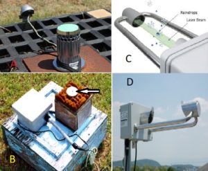
Nowadays, we use disdrometers:

• Impact (A,B): the instrument transforms the vertical momentum of impacting drops into electric pulses whose amplitude is a function of the drop diameter.
• Laser  (C,D): the instrument transforms the laser beam attenuation due to the passage of a rain drop into the drop diameter. These disdrometrers are also called Laser Precipitation Monitors.

Disdrometers do not report the diameter of each drop as a continuous variable, but they divide the range of possible diameter in classes (intervals), and count the number of drop for each class in a given time interval (integration time): usually 1 minute. Disdrometers catchment area is roughly in the range [50,100] cm$^2$ depending on instrument model.

Cloud versus Ground

The great majority of disdrometric observations occur on Earth’s surface, with only few cases of airborne observations (with laser disdrometers). Therefore disdrometers measurements can be used to estimate the rain drop spectrum at the ground. This “ground” spectrum is not equal to the “cloud” one as rain drops of different size fall at different speed. However, one can  estimate the cloud spectrum from the ground spectrum if the relationship between the drop diameter and the falling speed is known.

Drop size distribution vs Spectrum

A great deal is known about the mechanisms of drop formation in the cloud and their effects on the distribution of drop sizes. As such, it is common in the hydro-meteorological community to describe the variability of drop diameters in terms of the drop size distribution $\mathcal{N}(D)$, namely  the concentration (m$^{-3}$mm$^{-1}$) per unit volume given a diameter $D$: $\mathcal{N}(D)\delta D$ is the number of drops per unit volume with diameter in the range $[D,D+\delta D]$. From a statistical point of view, it would formally more “proper” to write:  

\begin{equation}\mathcal{N}(D)=N_{V}f(D)\end{equation}

where $N_{V}$ is the number of drop per unit volume and $f(D)$ is the probability density function of drop diameters or cloud spectrum. The function $f(D)$ is what a person with a “statistical/statistics” background would properly call the cloud “drop size distribution” or cloud spectrum: welcome to interdisciplinary science.  

If you know the terminal velocity $v(D)$ of  drop as a function of its diameter $D$, you can calculate from the number of drops with diameter $[D,D+\delta D]$ in the range passing through an Area of size $A$ ($m^2$) in a given time $T$ ($s$) as

\begin{equation}\label{eq:cloudvsground}Np(D)=N_{V}f(D) \times [AT] \times v(D)=N_{V}f(D) \times [AT] \times 3.78D^{0.67}\end{equation}

where $v(D)=3.78D^{0.67}$ $m/s$ (Atlas & Ulbrich) is the commonly accepted  formula for terminal velocity.

A ground based disdrometer measures  $Np(D)$ ($A$ being the catchment area of the instrument and $T$ its integration time), and one can invert the above equation to obtain $N_{V}f(D)$. 

Statistical description of rainfall

A statistical description of rainfall can be accomplished using either  the couple $(N_{V},f(D))$ (cloud description) or the couple $(N,p(D))$ (ground description). The two descriptions are equivalent and one can switch between them using Eq.(2).

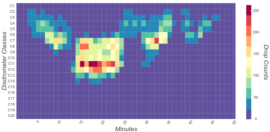
We  use the “ground” description $(N,p(D))$. Below are examples of what consecutive minutes of disdrometer measurements look like: (A) text format, (B) heat map. Looking at the heat map you can almost “listen” to the “pulsating” nature of rain: rain fall intensity increase (minutes 1-13), it reaches a plateau (minutes 14-24), and then slow down again (minute> 24) with a small peak in intensity (minutes 30-35).

Disdrometers “quantize” drop diameters in to classes. Therefore, the ground spectrum estimated from a disdrometer count will be a step function (the same value for all the diameters inside a given class):

\begin{equation}p(D)=\frac{n_{j}}{N\Delta_{j}}I_{j}(D)\end{equation}

where $N$ is the total number fo drops in the integration interval, $n_{j}$ and $\Delta_{j}$ are, respectively, the number of drops and the size of the of the $j-$th disdrometer class, while $I_{j}(D)=1$ if $D$ is inside the range of the $j-$th disdrometer class and  $I_{j}(D)=$ otherwise (a step function) .

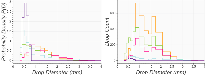
Moreover the size of disdrometer drop classes is not uniform: therefore the disdrometer counts are not proportional to the corresponding probability density function $p(D)$. The figure below illustrates this point, and also the natural variability of the shape of $p(D)$ (more about the variability in the second installment)

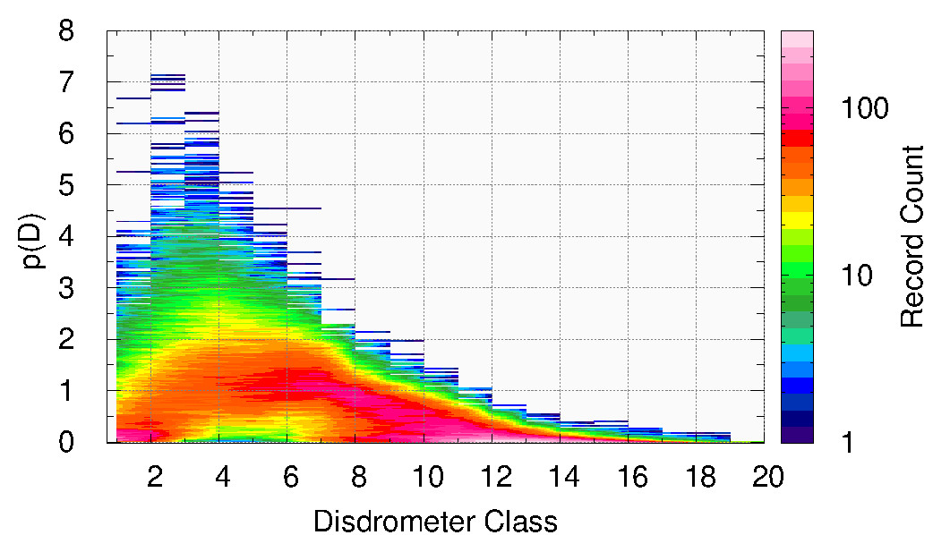
Finally to “stress” the point on the variability of the rain drop spectrum, Let us consider almost 4  months of 1-minute disdrometer data collected in Darwin, Australia. For each disdrometer class, we count how many 1-minute records have a particular value for the probability density function $p(D)$. The results are reported in the below figure: e.g. for the fourth disdrometer class the probability density function can essentially assume any value in the interval [0,4].

Material

• Disdrometer data analysis is performed with the disdrorain python package that you can find in my github repository.
• Figure are generated with python packages Bokeh, and with the software Gnuplot.
• Disdrometer data are the one collected in Darwin (AUS) as part of the Tropical Warm Pool International Cloud Experiment.

References & Additional reads

• Atlas & Ulbrich: “Path- and Area-Integrated Rainfall Measurement by Microwave Attenuation in the 1–3 cm Band”. The formula for $v(D)$ is Eq.(8) as expressed in m/s.
• “Precipitation: Theory, Measurement and Distribution”: as the title suggests, this book provides a good background on the basics of precipitation theory, and its measurement and distribution.